⬅️

Physics

Introduction to Physics

Physics is the natural science that studies matter, its fundamental constituents, its motion and behavior through space and time, and the related entities of energy and force. The most famous equation demonstrating the mass-energy equivalence is:

$$E = mc^2$$

School Physics

Subtopics can be accessed from the sidebar

Units & Measurement

The foundational study of physical quantities, the international system of units (SI), dimensional analysis, and error calculation.

Motion in a Straight Line

The kinematics of objects moving in one dimension, exploring concepts like displacement, velocity, and acceleration over time.

Motion in a Plane

The study of two-dimensional kinematics, introducing vectors, projectile motion, and uniform circular motion.

Laws of Motion

Newton's three fundamental laws governing classical mechanics, including inertia, force, and action-reaction pairs.

Work, Energy and Power

The relationship between forces applied over a distance, the conservation of mechanical energy, and the rate of doing work.

Center of Mass and Collision

Analyzing systems of particles, defining the center of mass, and understanding the conservation of momentum in elastic and inelastic collisions.

Rotational Motion

The kinematics and dynamics of rigid bodies rotating about a fixed axis, including torque and angular momentum.

Gravitation

Newton's law of universal gravitation, Kepler's laws of planetary motion, and the concept of gravitational potential energy.

Properties of Matter

The mechanical properties of solids and fluids, including elasticity, surface tension, viscosity, and Bernoulli's principle.

Heat and Thermodynamics

The study of thermal expansion, calorimetry, heat transfer, and the fundamental laws of thermodynamics governing energy and entropy.

Oscillations

The physics of periodic motion, focusing heavily on Simple Harmonic Motion (SHM) in springs and pendulums.

Waves

The propagation of mechanical disturbances through mediums, exploring concepts like wavelength, frequency, superposition, and the Doppler effect.

Electrostatics

Electrostatics deals with the study of forces, fields, and potentials arising from static charges. This forms the foundation for electromagnetism.


1. Coulomb's Law

Coulomb's law states that the electrostatic force between two point charges is directly proportional to the product of the magnitudes of charges and inversely proportional to the square of the distance between them.

$$F = \frac{1}{4\pi\epsilon_0} \frac{q_1 q_2}{r^2}$$

Vector Form: The force on charge $q_2$ due to $q_1$ is given by:

$$\vec{F}_{12} = \frac{1}{4\pi\epsilon_0} \frac{q_1 q_2}{r^2} \hat{r}_{12}$$

Where $\epsilon_0$ is the permittivity of free space ($\approx 8.854 \times 10^{-12} \text{ C}^2\text{N}^{-1}\text{m}^{-2}$).


2. Electric Field and Potential

Electric Field (E): The electrostatic force experienced per unit positive test charge. For a point charge $q$ at a distance $r$:

$$\vec{E} = \frac{\vec{F}}{q_0} = \frac{1}{4\pi\epsilon_0} \frac{q}{r^2} \hat{r}$$

Electric Potential (V): The work done by an external force in bringing a unit positive charge from infinity to a point. For a point charge $q$:

$$V = \frac{1}{4\pi\epsilon_0} \frac{q}{r}$$

Relation between E and V: The electric field is the negative gradient of the electric potential.

$$\vec{E} = -\nabla V = -\left( \frac{\partial V}{\partial x}\hat{i} + \frac{\partial V}{\partial y}\hat{j} + \frac{\partial V}{\partial z}\hat{k} \right)$$


3. Electric Dipole

A system of two equal and opposite charges ($+q$ and $-q$) separated by a small distance ($2a$). The dipole moment $\vec{p}$ is a vector directed from $-q$ to $+q$ with magnitude $p = q(2a)$.

Torque in a Uniform Electric Field: When placed in a uniform field $\vec{E}$, the net force is zero, but the charges experience equal and opposite forces creating a couple. The torque ($\tau$) is the cross product of dipole moment and electric field:

$$\vec{\tau} = \vec{p} \times \vec{E} \implies \tau = pE \sin\theta$$

Potential Energy of a Dipole: The work done in rotating a dipole from an angle $\theta_1$ to $\theta_2$ is stored as potential energy ($U$). Taking standard reference at $90^\circ$:

$$U = -\vec{p} \cdot \vec{E} = -pE \cos\theta$$


4. Gauss's Law

Electric Flux ($\Phi_E$): The measure of electric field lines crossing a given surface area. For a uniform electric field and a planar area vector $\vec{A}$:

$$\Phi_E = \int \vec{E} \cdot d\vec{A}$$

Gauss's Theorem: The total electric flux through any closed surface is equal to $1/\epsilon_0$ times the net charge enclosed by the surface.

$$\oint \vec{E} \cdot d\vec{A} = \frac{q_{\text{enclosed}}}{\epsilon_0}$$

Exam Note: Gauss's Law is primarily useful for finding electric fields for highly symmetric charge distributions (e.g., infinite line charge, infinite plane sheet, spherical shells).

Current Electricity

The study of electric current in conductors, encompassing the dynamics of moving charges, resistance, and complex circuit analysis.


1. Electric Current and Drift Speed

Electric current is the rate of flow of charge. In a conductor, electrons move with an average velocity called drift speed ($v_d$) when an electric field is applied.

The relation between current ($I$) and drift speed is:

$$I = neAv_d$$

Where $n$ is number density of electrons, $e$ is elementary charge, and $A$ is the cross-sectional area.


2. Ohm's Law and Resistivity

Ohm's Law states that voltage across a conductor is directly proportional to the current flowing through it, provided temperature remains constant.

$$V = IR$$

The microscopic form relating current density ($\vec{J}$) and electric field ($\vec{E}$) is $\vec{J} = \sigma\vec{E}$, where $\sigma$ is conductivity.

Temperature Dependence of Resistivity: Resistivity ($\rho$) changes with temperature ($T$) according to the empirical formula:

$$\rho = \rho_0 [1 + \alpha(T - T_0)]$$

Where $\alpha$ is the temperature coefficient of resistivity.


3. Kirchhoff's Laws

Essential for analyzing complex electrical circuits:

  • Junction Rule (KCL): The algebraic sum of currents at any junction is zero ($\sum I = 0$). This is based on the conservation of charge.
  • Loop Rule (KVL): The algebraic sum of changes in potential around any closed loop is zero ($\sum \Delta V = 0$). This is based on the conservation of energy.

4. Wheatstone Bridge

A specific arrangement of four resistors used to determine an unknown resistance. In the balanced condition (no current through the galvanometer), the ratio of the arms is equal:

$$\frac{R_1}{R_2} = \frac{R_3}{R_4}$$

Capacitors

Devices designed to store electrical energy and charge in an electric field.


1. Capacitor and Capacitance

Capacitance ($C$) is the ratio of the charge ($Q$) on either conductor to the potential difference ($V$) between them.

$$C = \frac{Q}{V}$$


2. Parallel-Plate Capacitor

The most common type of capacitor. For plates of area $A$ separated by a distance $d$ in a vacuum, the calculation of capacitance yields:

$$C_0 = \frac{\epsilon_0 A}{d}$$

With a Dielectric: When a dielectric material of constant $K$ fills the space, the capacitance increases:

$$C = K C_0 = \frac{K \epsilon_0 A}{d}$$


3. Combination of Capacitors

Capacitors can be grouped in circuits to achieve a desired equivalent capacitance:

  • Series Combination: Charge remains constant across all capacitors. The equivalent capacitance is given by:

    $$\frac{1}{C_{eq}} = \frac{1}{C_1} + \frac{1}{C_2} + \dots + \frac{1}{C_n}$$

  • Parallel Combination: Voltage remains constant across all capacitors. The equivalent capacitance is given by:

    $$C_{eq} = C_1 + C_2 + \dots + C_n$$


4. Energy Stored and Energy Density

The work done in charging a capacitor is stored as electrostatic potential energy ($U$). It can be calculated as:

$$U = \frac{1}{2}CV^2 = \frac{Q^2}{2C} = \frac{1}{2}QV$$

Energy Density ($u$): The energy stored per unit volume in the electric field between the plates is:

$$u = \frac{1}{2}\epsilon_0 E^2$$

Moving Charges and Magnetism

This section explores the Definition of Magnetic Field $\vec{B}$, the Relation between Electric and Magnetic Fields, and the Motion of a Charged Particle in a Uniform Magnetic Field.


1. Magnetic Force

  • On a moving charge: A charge $q$ moving with velocity $\vec{v}$ in a magnetic field $\vec{B}$ experiences a force given by $\vec{F} = q(\vec{v} \times \vec{B})$.
  • On a current-carrying wire: The Magnetic Force on a Current-carrying Wire of length $\vec{l}$ and current $I$ is calculated as $\vec{F} = I(\vec{l} \times \vec{B})$.
  • Torque: The Torque on a Current Loop is given by $\vec{\tau} = \vec{m} \times \vec{B}$, where $\vec{m}$ is the magnetic moment.

2. Magnetic Field due to a Current

  • Biot-Savart Law: Determines the magnetic field $d\vec{B}$ generated by a differential current element $Id\vec{l}$.

    $$d\vec{B} = \frac{\mu_0}{4\pi} \frac{I d\vec{l} \times \hat{r}}{r^2}$$

  • Ampere's Law: States that the line integral of the magnetic field around any closed loop is equal to $\mu_0$ times the enclosed current.

    $$\oint \vec{B} \cdot d\vec{l} = \mu_0 I_{\text{enc}}$$

3. Key Applications

  • Derivations for the Magnetic Field due to Current in a Straight Wire and the Field due to a Circular Current.
  • Calculating the Force between Parallel Currents, which is historically used to define the Ampere.
  • Determining the magnetic field inside a Solenoid and a Toroid using Ampere's Law.

Magnetism and Matter

This chapter studies Permanent Magnets, including Magnetic Poles and Bar Magnets, and the underlying Magnetic Properties of Matter.


1. Permanent Magnets & Earth's Field

  • Bar Magnets: Core concepts include calculating the Torque on a Bar Magnet Placed in a Magnetic Field, the Magnetic Field due to a Bar Magnet, and understanding Magnetic Scalar Potential.
  • Earth's Magnetism: Encompasses Terrestrial Magnetism, the Determination of Dip at a Place, and identifying a Neutral Point.
  • Gauss's Law for Magnetism: States that the net magnetic flux through any closed surface is zero ($\oint \vec{B} \cdot d\vec{A} = 0$), implying magnetic monopoles do not exist.

2. Measuring Instruments

  • Operational principles of the Tangent Galvanometer, Moving-coil Galvanometer, and Deflection Magnetometer.
  • Galvanometer modifications involve calculating and applying a Shunt resistor.

3. Magnetic Properties of Matter

  • Key Metrics: Defining Magnetization of Materials: Intensity of Magnetization, Magnetic Intensity $H$, Magnetic Susceptibility, and Permeability.
  • Classification: Studying the Properties of Dia-, Para- and Ferromagnetic Substances.
  • Laws and Effects: Exploring Curie's Law, Hysteresis, and the practical differences between Soft Iron and Steel.

Electromagnetic Induction

The study of how changing magnetic environments can induce electromotive forces and currents.


1. Fundamental Laws

  • Faraday's Law of Electromagnetic Induction: The induced emf is equal to the negative rate of change of magnetic flux.

    $$\mathcal{E} = -\frac{d\Phi_B}{dt}$$

  • Lenz's Law: Dictates that the direction of the induced current opposes the change in magnetic flux that produced it, aligning with the conservation of energy.
  • Origin: Explaining The Origin of Induced emf and the formation of Eddy Current in bulk conductors.

2. Induction and Circuits

  • Types of Induction: Definitions and formulas for Self-induction and Mutual Induction.
  • Energy: The Energy Stored in an Inductor is given by the formula $U = \frac{1}{2}LI^2$.
  • Transient Responses: Formulating the Growth and Decay of Current in an $LR$ Circuit.
  • Applications: Understanding the mechanics of the Induction Coil.

Alternating Current

Electrical circuits where the current periodically reverses direction, analyzing impedance, resonance, and transformers.

Electromagnetic Waves

The unified propagation of electric and magnetic fields through space, and the complete electromagnetic spectrum.

Geometrical Optics

The behavior of light utilizing ray approximations to study reflection, refraction, lenses, mirrors, and optical instruments.

Wave Optics

The phenomena of light that require a wave model to explain, including interference (Young's double-slit), diffraction, and polarization.

Atoms and Nuclei

Rutherford and Bohr models of the atom, atomic spectra, and the composition, stability, and radioactive decay of atomic nuclei.

Dual Nature of Radiation and Matter

The quantum mechanical reality that light exhibits particle properties (photons) and matter exhibits wave properties (de Broglie waves).

Semiconductor Electronics

The physics of materials with conductivity between insulators and conductors, forming the basis of diodes, transistors, and modern computing.
Dynamics

To simplify the study of dynamical systems we will divide it into six main parts depending on weather we are studying single/many body, at low/high speeds and if we are in the quantum/classical limits. For three out of four forces we have experimentally verified Quantum Theory. For the forth force of Gravity we a very beautiful classical theory by Einstein whose Quantum Part is yet to be discovered experimentally but still we have really a very strong candidate called String Theory which is mathematically consistent and brings all forces unders one formalism. For now we will be exploring these experimentally verified regims :

  1. Single Body Non-Relativistic Classical Physics (CM)
  2. Many Body Non-Relativistic Classical Physics (SM)
  3. Single Body Non-Relativistic Quantum Physics (QM)
  4. Many Body Non-Relativistic Quantum Physics (CMP)
  5. Single Body Relativistic Classical Physics (STR+GR)
  6. Many-Body Relativistic Quantum Physics (QFT)

In any kind of Dynamics, its helpful define the SYSTEM, the STATE and EVOLUTION. In Newtonian Mechanics, we defined the SYSTEM as the particle acted on by a Force whose STATE (Initial) was given by pair of position and velocity vectors and finally using Newtons Laws F=ma (solving this differential equation), we can get the position and velocity at later times (final state). We can extend this idea to our six divisions.

System Framework 1. CM 2. SM 3. QM 4. CMP 5. STR+GR 6. QFT
The System A low-speed particle A probability distribution (ensemble) A wavefunction An interacting many-body lattice A massive body in curved spacetime A quantized field
State Variables (State) $$(\mathbf{x}, \mathbf{p})$$ $$\rho(\mathbf{q}, \mathbf{p})$$ $$|\psi\rangle$$ $$|\Psi\rangle$$ $$g_{\mu\nu}, x^\mu(\tau)$$ $$\hat{\phi}(x), |0\rangle$$
Dynamical Equation (Evolution) $$m\ddot{\mathbf{x}} = -\nabla V$$ $$\frac{\partial \rho}{\partial t} = \{H, \rho\}$$ $$i\hbar\frac{\partial}{\partial t}|\psi\rangle = \hat{H}|\psi\rangle$$ $$\hat{H} = -t \sum_{\langle i,j \rangle, \sigma} (\hat{c}_{i\sigma}^\dagger \hat{c}_{j\sigma} + h.c.) + U \sum_i \hat{n}_{i\uparrow} \hat{n}_{i\downarrow}$$ $$R_{\mu\nu} - \frac{1}{2}Rg_{\mu\nu} = \frac{8\pi G}{c^4} T_{\mu\nu}$$ $$\mathcal{L} = \bar{\psi}(i\gamma^\mu\partial_\mu - m)\psi$$

$$...$$

Simulating Hubbard Model using Exact Diagonalization and Quantum Computation

Second Quantization

In formulating quantum mechanics from classical mechanics, we elevate the dynamical variables $q_i$'s and $p_i$'s to operators and define a commutation relation between them as $[q_i,p_i]=i\hbar$. This is called First Quantization.

When we elevate the wavefunction $\psi(r)$ itself to operator also known as Field Operator $\vu{\psi}(r)$, this formulation is called Second Quantization. Similar to how a $q_i$ has a canonical conjugate as $p_i$, the field operator $\vu{\psi}(r)$ has $\vu{\psi}^{\dagger}(r)$ and they have a commutation relation between them given as $[\vu{\psi}(r_1),\vu{\psi}^{\dagger}(r_2)]=\delta(r_1 - r_2)$ for Bosons and Anti-commutation relation for Fermions i.e. $\{\vu{\psi}(r_1),\vu{\psi^{\dagger}}(r_2)\}=\delta(r_1 - r_2)$.

This field operator which is function of space and time in one dimension in general is defined as :

$$ \vu{\psi}(r)=\sum_n c_n \phi_n(r) $$

where, $\phi_n(x)$ is the usual first quantization wavefunction and $c_n$ is the annihilation operator. Similarly its canonical conjugate is defined as :

$$ \vu{\psi}^{\dagger}(r)=\sum_n c_n^{\dagger} \phi_n^*(r) $$

where, $\phi_n^*(x)$ is the complex conjugate of the wave function and $c_n^{\dagger}$ is the creation operator.

These creation and annhilation operators will act on the STATE of the system which is called the "Fock Space". which we will denote by :

$$ \ket{n_1, n_2, n_3, ..., n_i, ... , n_N} $$

where, $n_i$ tells us the number of particles present at the ith state (first quantization wavefunction).

A "Vaccum State", where physically there are no particles present in our space is $\ket{0, 0, ..., 0}$. So as an example if we act $c_1^{\dagger}$ on the vaccum state, we get $\sqrt{2} \ket{1, 0, ..., 0}$ and $c_1$ acting on vacuum state will give us zero.

Disclaimer

We have borrowed the action of ladder operators from first quantization from the harmonic oscillator but physically these are two different operators. In first quantization the creation ladder operator will change the $\ket{n}$ to $\ket{n+1}$ by and factor of $\sqrt{n+1}$ and annihilation operator will change $\ket{n}$ to $\ket{n-1}$ by a factor of $\sqrt{n}$.


System

If we look at atoms whose outermost shell is the s orbital then their wave function is not localized i.e. of the form $\psi = e^{i(k\cdot r)}$ (The probability of finding the particle is equally like everywhere). But if we take a look at the atoms whose outermost electrons lie in the d orbital. These wavefunctions are bound to the atom and they have localization around the ion. But the localization is not strong enough for them so as to stop them from tunneling the neighbouring atoms and occupy and empty state present. Now given the fixed number of such electrons and fixed number of sites, the system will choose a state such that the total energy of the system is minimized. The dynamics of such materials can be modelled by what is called the Hubbard Model whose Hamiltonian can be written as:

$$ H = -t \sum_{i,\sigma} c_{i,\sigma}^\dagger c_{i+1,\sigma} + h.c + U \sum_{i}^n {n_{i\uparrow}} {n_{i\downarrow}} $$

where:

  • $c_{i,\sigma}^\dagger$: The creation operator for an electron with spin $\sigma$ ($\uparrow$ or $\downarrow$) at site $i$.
  • $c_{i,\sigma}$: The annihilation operator for an electron with spin $\sigma$ at site $i$.
  • $t$: The hopping amplitude, representing the kinetic energy of an electron hopping between nearest-neighbor sites.
  • $n_{i\sigma} = c_{i,\sigma}^\dagger c_{i,\sigma}$: The number operator for electrons with spin $\sigma$ at site $i$.
  • $U$: The on-site Coulomb interaction energy between two electrons of opposite spins ($\uparrow$ and $\downarrow$) at the same site.

It is an extension of the Tight Binding Approximation for single band and inclusion of electron-electron repulsion. Hubbard Model was introduced in order to explain the insulating behaviour of partially filled Transition Metal Oxide like TiO. Not only that in the limiting behaviour where the repulsion between electrons is more than the tunneling term, the electrons tends to localize on sites having same spin and hence show ferromagnetism.


State

We are going to choose our basis state as what is called Wernier Wave Functions (they are fourier transforms of conventional Bloch States) which will give us the state of ONE electron localized on ONE particular site labelled by index i.

$$ W_\gamma(\vec{r}-\vec{R_i}) = \frac{1}{\sqrt{N}} \sum_{k} e^{-i \vec{k}\cdot\vec{R_i}} \phi_{k,\gamma}(\vec{r}) $$

Here, $\gamma$ is the band index, $\vec{R}$ is the ionic position vector, $\phi(\vec{r})$ is the Bloch wave function. We can then also define a ortho normality between states of different sites.

$$ \bra{W_n(\vec{r}-\vec{R_i})}\ket{W_n(\vec{r}-\vec{R_j})} = \delta_{R_i,R_j} $$

Since this is a fermionic system, each site can have either one up spin or one down spin or both one up and one down spin. In order to denote the state of the system i.e. all sites at once we will use the notation as follows:

$$ \ket{\uparrow} \quad \ket{\downarrow} \quad \ket{\uparrow\downarrow} $$

Exact Diagonalization

2 Sites 2 Electrons

All possible states for 2 sites and 2 electrons will look like:

$$ \ket{\uparrow,\uparrow} \quad \ket{0,\uparrow\downarrow} \quad \ket{\uparrow, \downarrow} \quad \ket{\downarrow,\uparrow} \quad \ket{\uparrow\downarrow, 0} \quad \ket{\downarrow,\downarrow} $$

The Hamiltonian for this system is:

$$ \begin{aligned} H = &-t ( c_{1\uparrow}^\dagger c_{2\uparrow} + c_{2\uparrow}^\dagger c_{1\uparrow} + c_{1\downarrow}^\dagger c_{2\downarrow} + c_{2\downarrow}^\dagger c_{1\downarrow} ) \\ &+ U ( n_{1\uparrow} n_{1\downarrow} + n_{2\uparrow} n_{2\downarrow} ) \end{aligned} $$

When we operate this Hamiltonian operator on all the six states we get:

$H \ket{\uparrow,\uparrow} = 0$

$H \ket{0,\uparrow\downarrow} = -t ( \ket{\uparrow, \downarrow} + \ket{\downarrow,\uparrow} ) + U (\ket{0,\uparrow\downarrow})$

$H \ket{\downarrow, \uparrow} = -t ( \ket{0,\uparrow\downarrow} + \ket{\uparrow\downarrow, 0} )$

$H \ket{\downarrow\uparrow, 0} = -t ( \ket{\downarrow,\uparrow} + \ket{\uparrow, \downarrow}) + U \ket{\uparrow\downarrow, 0}$

$H \ket{\downarrow,\downarrow} = 0$

From this we can easily get the matrix element. For t = 1, U = 1:

$$ \begin{bmatrix} 0 & 0 & 0 & 0 & 0 & 0 \\ 0 & 1 & -1 & -1 & 0 & 0 \\ 0 & -1 & 0 & 0 & -1 & 0 \\ 0 & -1 & 0 & 0 & -1 & 0 \\ 0 & 0 & -1 & -1 & 1 & 0 \\ 0 & 0 & 0 & 0 & 0 & 0 \end{bmatrix} $$

On Diagonalizing this matrix numerically using LAPACK library function, we get Eigenvalues : 2.56, -1.56, 1, 0, 0, 0. The Ground State Energy as -1.56.


Nagaoka's Theorem

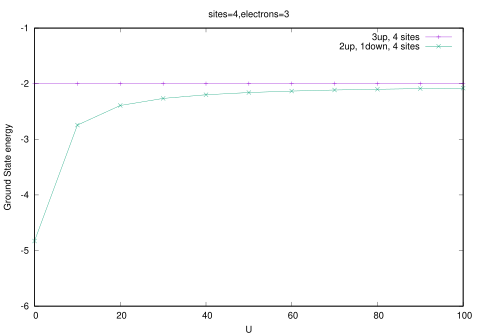
Statement: In Hubbard Model, the relative ground state in the sector with one unoccupied site is maximally FERROMAGNETIC for large U.

Nagaoka's Theorem Graph

For 4 sites and 3 electrons we have plotted U v/s Ground State Energies

In operational sense it means that if we take one less than half filled sites, then for large value of U (interaction between electrons on same site), the ground state of the system will be Ferromagnetic and spins will try to allow themselves in one direction. The Hubbard model can become equivalent to the Heisenberg model in the limit of strong electron-electron interactions (U) compared to the kinetic energy (t), particularly in the limit of large U and at half-filling of the electron density (one electron per lattice site). In this regime, virtual hopping processes are suppressed due to the high energy cost of double occupancy, leading to an effective spin-spin interaction between localized electrons. Under these conditions, the Hubbard model effectively reduces to the Heisenberg model, where the kinetic energy terms are neglected, and the dominant interactions are described by spin operators.


Quantum Simulation

Qubit

In quantum computing, the fundamental unit of information is the qubit, which can exist in a superposition of two basis states $|0\rangle$ and $|1\rangle$. The state of a single qubit is generally represented as:

$$ |\psi\rangle = \alpha |0\rangle + \beta |1\rangle $$

where:

  • $|0\rangle$ and $|1\rangle$ are the computational basis states, analogous to the classical binary states.
  • $\alpha$ and $\beta$ are complex numbers representing the probability amplitudes of the respective basis states.
  • The coefficients satisfy the normalization condition $|\alpha|^2 + |\beta|^2 = 1$, ensuring the total probability is conserved.
Bloch Sphere

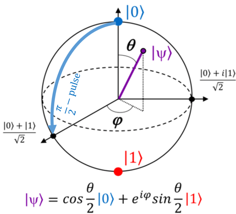
Bloch Sphere

A general qubit in this 3 dimensional space can then be written as:

$$ |\psi\rangle = \cos\left(\frac{\theta}{2}\right) |0\rangle + e^{i\phi} \sin\left(\frac{\theta}{2}\right) |1\rangle $$

where:

  • $\theta$ is the polar angle ($0 \leq \theta \leq \pi$).
  • $\phi$ is the azimuthal angle ($0 \leq \phi < 2\pi$).
  • The coefficients $\alpha$ and $\beta$ are parameterized as: $\alpha = \cos\left(\frac{\theta}{2}\right)$ and $\beta = e^{i\phi} \sin\left(\frac{\theta}{2}\right)$.

In the context of quantum computing, the $|0\rangle$ and $|1\rangle$ states of a qubit can be mapped to the physical occupation states of a fermionic site:

  • $|0\rangle$: Represents the absence of a particle (no occupation) at the site.
  • $|1\rangle$: Represents the presence of a particle (occupied) at the site.

For the Hubbard Model, which includes both spin-up ($\uparrow$) and spin-down ($\downarrow$) fermions at each site, the Hilbert space of a single site is expanded to account for four possible states:

  • $|00\rangle$: No particles at the site.
  • $|01\rangle$: A spin-down ($\downarrow$) particle occupies the site.
  • $|10\rangle$: A spin-up ($\uparrow$) particle occupies the site.
  • $|11\rangle$: Both spin-up ($\uparrow$) and spin-down ($\downarrow$) particles occupy the site.

Jordan Wigner Transformation

The Jordan-Wigner Transformation allows fermionic creation and annihilation operators to be represented as spin operators. Specifically, the creation and annihilation operators at site $j$ are expressed as:

$$ \begin{aligned} c_{j}^\dagger &= \frac{1}{2} \left( \prod_{k=1}^{j-1} Z_k \right) (X_j - i Y_j) \\ c_{j} &= \frac{1}{2} \left( \prod_{k=1}^{j-1} Z_k \right) (X_j + i Y_j) \end{aligned} $$

Variational Quantum Eigensolver

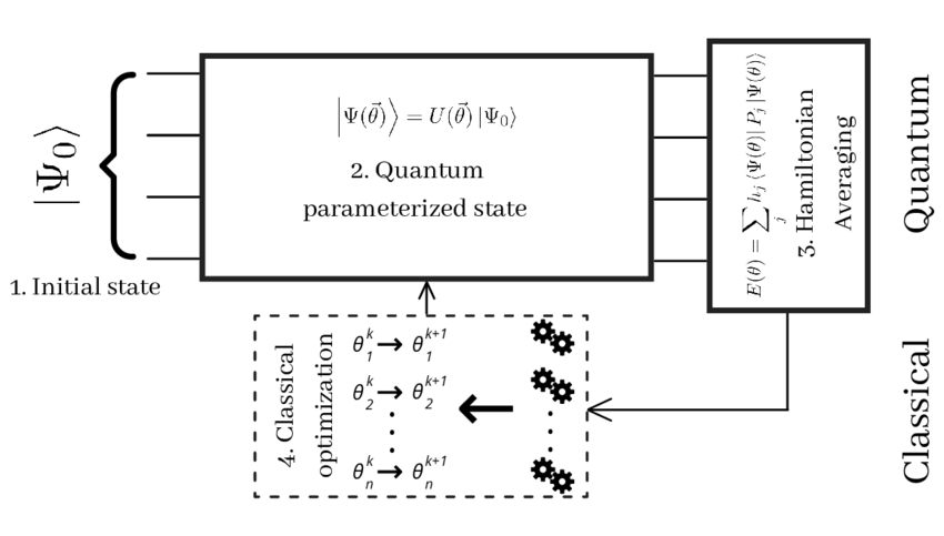
The ground state energy of a quantum system can be expressed as the expectation value of the Hamiltonian $H$ with respect to a trial wavefunction $|\psi(\theta)\rangle$, parameterized by $\theta$. Mathematically, this is given by:

$$ E(\theta) = \langle \psi(\theta) | H | \psi(\theta) \rangle $$

where $E(\theta)$ represents the energy for a given parameter set $\theta$. The Variational Quantum Eigensolver aims to minimize this energy by optimizing the parameters $\theta$ such that:

$$ E_{\text{ground}} = \min_{\theta} \langle \psi(\theta) | H | \psi(\theta) \rangle $$
Variational Quantum Eigensolver

Variational Quantum Algorithm Eigensolver

The Variational Quantum Eigensolver (VQE) is a hybrid quantum-classical algorithm designed to find the ground state energy of quantum systems. The algorithm minimizes the expectation value of the Hamiltonian $H$, which represents the system's energy operator, to identify the lowest possible energy state.